Getting Started with Oracle Cloud Infrastructure Data Flow

This tutorial introduces you to Oracle Cloud Infrastructure Data Flow, a service that lets you run any Apache Spark Application  at any scale with no infrastructure to deploy or manage.

If you've used Spark before, you'll get more out of this tutorial, but no prior Spark knowledge is required. All Spark applications and data have been provided for you. This tutorial shows how Data Flow makes running Spark applications easy, repeatable, secure, and simple to share across the enterprise.

In this tutorial you learn:
  1. How to use Java to perform ETL in a Data Flow Application .
  2. How to use SparkSQL in a SQL Application.
  3. How to create and run a Python Application to perform a simple machine learning task.

You can also perform this tutorial using spark-submit from CLI or using spark-submit and Java SDK.

Data Flow Advantages
Here's why Data Flow is better than running your own Spark clusters, or other Spark Services out there.
  • It's serverless, which means you don't need experts to provision, patch, upgrade or maintain Spark clusters. That means you focus on your Spark code and nothing else.
  • It has simple operations and tuning. Access to the Spark UI is a click away and is governed by IAM authorization policies. If a user complains that a job is running too slow, then anyone with access to the Run can open the Spark UI and get to the root cause. Accessing the Spark History Server is as simple for jobs that are already done.
  • It is great for batch processing. Application output is automatically captured and made available by REST APIs. Do you need to run a four-hour Spark SQL job and load the results in your pipeline management system? In Data Flow, it's just two REST API calls away.
  • It has consolidated control. Data Flow gives you a consolidated view of all Spark applications, who is running them and how much they consume. Do you want to know which applications are writing the most data and who is running them? Simply sort by the Data Written column. Is a job running for too long? Anyone with the right IAM permissions can see the job and stop it.
There is a table of nine columns and three rows. The columns are Name, Language, Status, Owner, Created, Duration, Total oCPU, Data Read, Data Written. The cells in all three rows are all populated. The names are Tutorial Example 1, Tutorial Example 2, and Tutorial Example 3. The languages for each are Java, Python, and SQL respectively. All three have a Status of Succeeded.

Before You Begin

To successfully perform this tutorial, you must have Set Up Your Tenancy and be able to Access Data Flow.

Set Up Your Tenancy

Before Data Flow can run, you must grant permissions that allow effective log capture and run management. See the Set Up Administration section of Data Flow Service Guide, and follow the instructions given there.

Accessing Data Flow
  1. From the Console, click the navigation menu to display the list of available services.
  2. Click Analytics & AI.
  3. From under Big Data, click Data Flow.
  4. Click Applications.

1. ETL with Java

An exercise to learn how to create a Java application in Data Flow

The steps here are for using the Console UI. You can complete this exercise using spark-submit from CLI or spark-submit with Java SDK.

Overview

The most common first step in data processing applications, is to take data from some source and get it into a format that's suitable for reporting and other forms of analytics. In a database, you would load a flat file into the database and create indexes. In Spark, your first step is to clean and convert data from a text format into Parquet format. Parquet is an optimized binary format supporting efficient reads, making it ideal for reporting and analytics. In this exercise, you take source data, convert it into Parquet, and then do a few interesting things with it. The dataset is the Berlin Airbnb Data dataset, downloaded from the Kaggle website under the terms of the Creative Commons CC0 1.0 Universal (CC0 1.0) "Public Domain Dedication" license.

There is a box labelled CSV Data, Easy to Read, Slow. An arrow flows to a box on the right labelled Parquet, Harder to Read, Fast. From there are two arrows, one to a box labelled SQL Queries and the other to a box labelled Machine Learning.

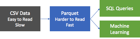
The data is provided in CSV format and the first step is to convert this data to Parquet and store it in object store for downstream processing. A Spark application, called oow-lab-2019-java-etl-1.0-SNAPSHOT.jar, is provided to make this conversion. The objective is to create a Data Flow Application which runs this Spark app, and run it with the correct parameters. Because you're starting out, this exercise guides you step by step, and provides the parameters you need. Later you need to provide the parameters yourself, so you must understand what you're entering and why.

Create the Java Application

Create a Data Flow Java Application from the Console, or with Spark-submit from the command line or using SDK.

Create the Java Application in the Console.

Create a Java application in Data Flow from the Console.

Create a Data Flow Application.

  1. Navigate to the Data Flow service in the Console by expanding the hamburger menu on the top left and scrolling to the bottom.
  2. Highlight Data Flow, then select Applications. Choose a compartment where you want the Data Flow applications to be created. Finally, click Create Application. Click Create Application
  3. Select Java Application and enter a name for the Application, for example, Tutorial Example 1. The Application page is displayed with the Create Application pull-out over the right-hand side. At the top is a section called General Information containing a text field called Name, and text field called Description. Then is a section called Resource configuration in which two text fields are visible. At the bottom are three buttons, Create, Save as stack, and Cancel.
  4. Scroll down to Resource Configuration. Leave all these values as their defaults. The Application page displayed with the Create Application pull-out over the right-hand side. The Resource Configuration section is visible. At the top is a drop-down list called Spark Version. Spark 3.0.2 is selected, but Spark 2.4.4 and Spark 3.2.1 are also listed. Below, but partially hidden by the list of Spark Versions is a text field called Select a pool. Then is a text field called Driver Shape. VM.Standard.E4.Flex is selected. Below and partially cropped is a section to customize the number of OCPUs. At the bottom are three buttons, Create, Save as Stack, and Cancel.
  5. Scroll down to Application Configuration. Configure the application as follows:
    1. File URL: is the location of the JAR file in object storage. The location for this application is:
      oci://oow_2019_dataflow_lab@idehhejtnbtc/oow_2019_dataflow_lab/usercontent/oow-lab-2019-java-etl-1.0-SNAPSHOT.jar
    2. Main Class Name: Java applications need a Main Class Name which depends on the application. For this exercise, enter
      convert.Convert
    3. Arguments: The Spark application expects two command line parameters, one for the input and one for the output. In the Arguments field, enter
      ${input} ${output}
      You're prompted for default values, and it's a good idea to enter them now.
    The Application page displayed with the Create Application pull-out over the right-hand side.The Application Configuration section is visible. At the top is a section called Select a file. A check box labeled Enter the file URL manually is seelcted. Next is a text field called File URL. It is populated with the path to the .jar file. Below is a text field called Main Class Name. It is populated with convert.Convert. Below is a text field called Arguments. It is populated with ${input} ${output}.
  6. The input and output arguments are:
    1. Input:
      oci://oow_2019_dataflow_lab@idehhejtnbtc/oow_2019_dataflow_lab/usercontent/kaggle_berlin_airbnb_listings_summary.csv
    2. Output:
      oci://<yourbucket>@<namespace>/optimized_listings

    Double-check the Application configuration, to confirm it looks similar to the following: The Application page displayed with the Create Application pull-out over the right-hand side. The Application Configuration section is visible. There is a text field called Arguments. It is populated with ${input} ${output}. Below are text fields for Parameters. There are two on the left that are greyed-out and populated with input and output respectively. Beside each is a text field labelled Default Value which are populated with the respective directories. Below is a section called Archive URI.

    Note

    You must customize the output path to point to a bucket in the tenant.
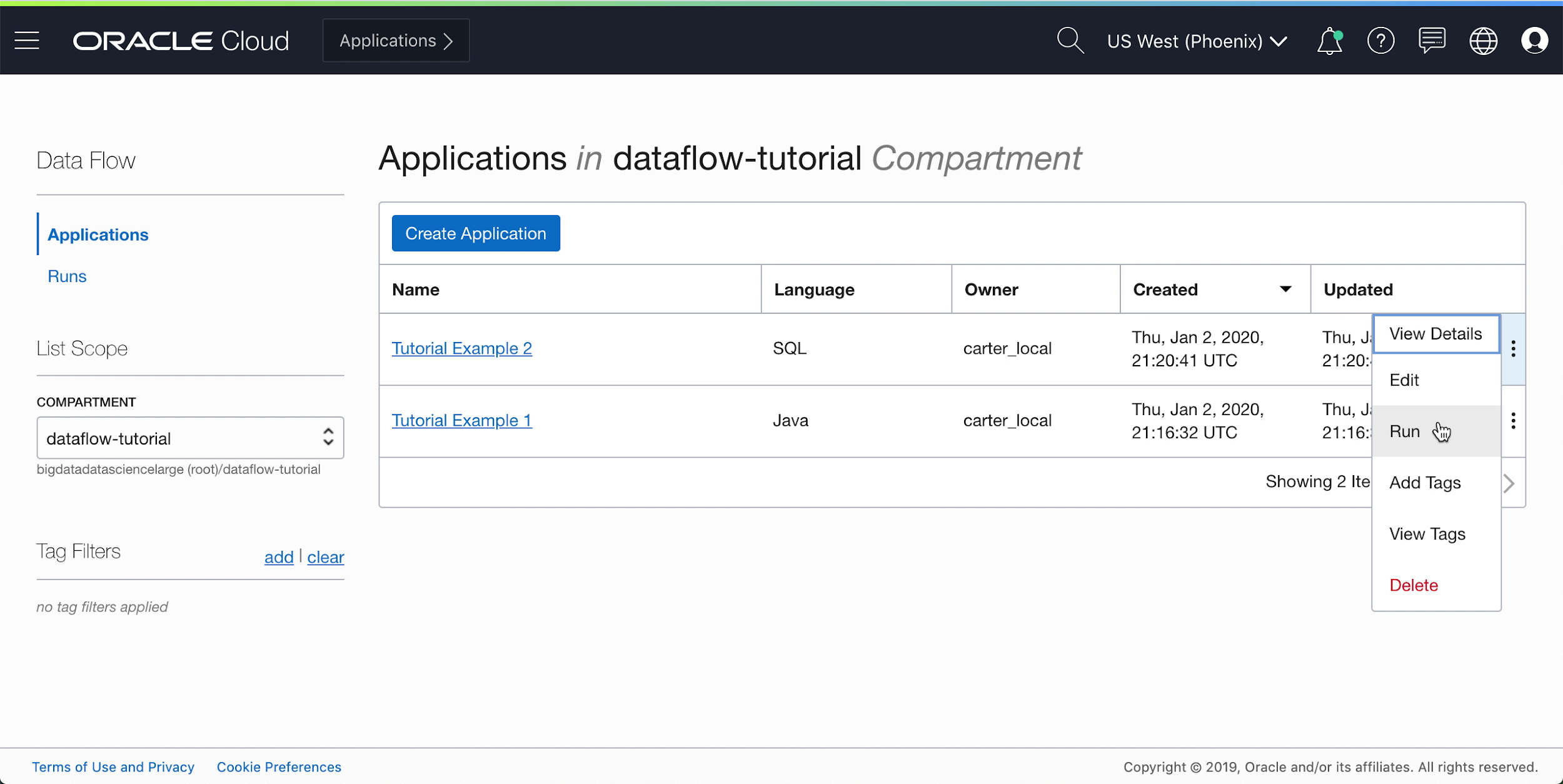
  7. When done, click Create. When the Application is created, you see it in the Application list. The Applications page. In the list of applications is one application. It consists of seven columns, Name, Language, Spark version, Application type, Owner, Created, and Updated. Name contains Tutorial Example 1. Language is set to Java. Spark version is set to 3.2.1. Application type is set to Batch. The other fields are populated according to who created the application, when it was created and when it was last updated (which in this case is the same date and time as Created).

Congratulations! You've created your first Data Flow Application. Now you can run it.

Create the Java Application Using Spark-Submit and CLI

Use spark-submit and CLI to create a Java Application.

  1. Set up your tenancy.
  2. If you don't have a bucket in Object Storage where you can save the input and results, you must create a bucket with a suitable folder structure. In this example, the folder structure is /output/tutorial1.
  3. Run this code:
    oci --profile <profile-name> --auth security_token data-flow run submit \
    --compartment-id <compartment-id> \
    --display-name Tutorial_1_ETL_Java \
    --execute '
        --class convert.Convert 
        --files oci://oow_2019_dataflow_lab@idehhejtnbtc/oow_2019_dataflow_lab/usercontent/kaggle_berlin_airbnb_listings_summary.csv 
        oci://oow_2019_dataflow_lab@idehhejtnbtc/oow_2019_dataflow_lab/usercontent/oow-lab-2019-java-etl-1.0-SNAPSHOT.jar \
        kaggle_berlin_airbnb_listings_summary.csv oci://<bucket-name>@<namespace-name>/output/tutorial1'
    If you have run this tutorial before, delete the contents of the output directory, oci://<bucket-name>@<namespace-name>/output/tutorial1, to prevent the tutorial failing.
    Note

    To find the compartment-id, from the navigation menu, click Identity and click Compartments. The compartments available to you're listed, including the OCID of each.
Create the Java Application Using Spark-Submit and SDK

Complete the exercise to create a Java application in Data Flow using spark-submit and Java SDK.

These are the files to run this exercise, and they're available on the following public Object Storage URIs:

  • Input files in CSV format:
    oci://oow_2019_dataflow_lab@idehhejtnbtc/oow_2019_dataflow_lab/usercontent/kaggle_berlin_airbnb_listings_summary.csv
  • JAR file:
    oci://oow_2019_dataflow_lab@idehhejtnbtc/oow_2019_dataflow_lab/usercontent/oow-lab-2019-java-etl-1.0-SNAPSHOT.jar
  1. Create a bucket in Object Storage where you can save the input and results.
  2. Run this code:
    public class Tutorial1 {
     
      String compartmentId = "<your-compartment_id>"; // Might need to change comapartment id
     
      public static void main(String[] ars) throws IOException {
        System.out.println("ETL with JAVA Tutorial");
        new Tutorial1().crateRun();
      }
     
      public void crateRun() throws IOException {
     
        // Authentication Using BOAT config from ~/.oci/config file
        final ConfigFileReader.ConfigFile configFile = ConfigFileReader.parseDefault();
     
        final AuthenticationDetailsProvider provider =
            new ConfigFileAuthenticationDetailsProvider(configFile);
     
        // Creating a Data Flow Client
        DataFlowClient client = new DataFlowClient(provider);
        client.setRegion(Region.US_PHOENIX_1);
        client.setEndpoint("http://<IP_address>:443");   // Might need to change endpoint
     
        // creation of execute String
        String executeString = "--class convert.Convert "
            + "--files oci://oow_2019_dataflow_lab@idehhejtnbtc/oow_2019_dataflow_lab/usercontent/kaggle_berlin_airbnb_listings_summary.csv "
            + "oci://oow_2019_dataflow_lab@idehhejtnbtc/oow_2019_dataflow_lab/usercontent/oow-lab-2019-java-etl-1.0-SNAPSHOT.jar "
            + "kaggle_berlin_airbnb_listings_summary.csv oci://<bucket_name>@<tenancy_name>/output/tutorial1";
     
        // Create Run details and create run.
        CreateRunDetails runDetails = CreateRunDetails.builder()
            .compartmentId(compartmentId).displayName("Tutorial_1_ETL_with_JAVA").execute(executeString)
            .build();
     
        CreateRunRequest runRequest = CreateRunRequest.builder().createRunDetails(runDetails).build();
        CreateRunResponse response = client.createRun(runRequest);
        GetRunRequest grq = GetRunRequest.builder().opcRequestId(response.getOpcRequestId()).runId(response.getRun().getId()).build();
        GetRunResponse gr = client.getRun(grq);
     
        System.out.println("Run Created!");
     
      }
    }
Run the Data Flow Java Application

Having created a Java application you can run it.

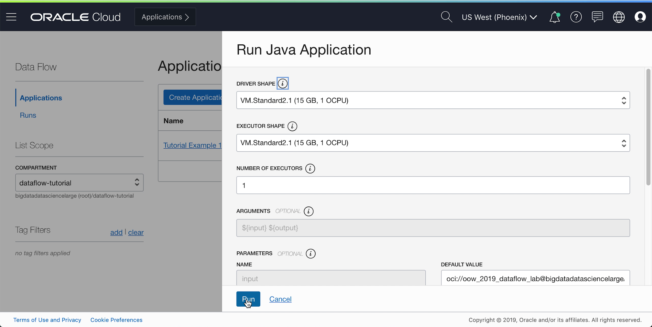
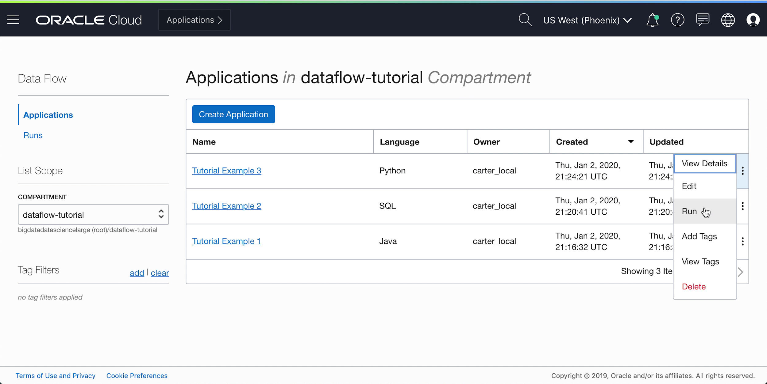
  1. If you followed the steps precisely, all you need to do is highlight your Application in the list, click Actions menu, and click Run.
  2. You're presented with the ability to customize parameters before running the Application. In your case, you entered the precise values ahead-of-time, and you can start running by clicking Run. The Run Java Application pull-out page displayed over the right-hand side of the Applications page. At the top is a drop-down list called Driver Shape; VM.Standard2.1 (15GB, 1 OCPU) is selected. Below is a drop-down list called Executor Shape; VM.Standard2.1 (15GB, 1 OCPU) is selected. Below is a text field labelled Number of Executors; it contains 1. Below is a text field called Arguments. It is greyed-out and contains ${input} ${output}. Below are two text fields side by side for parameters. The first is called Name and is greyed-out, but contains input. The other is called Default Value and contains the input directory, but can be edited. There is a scroll bar to the right which is at the top position. At the bottom of the screen are two buttons, Run and Cancel. Run is about to be clicked.
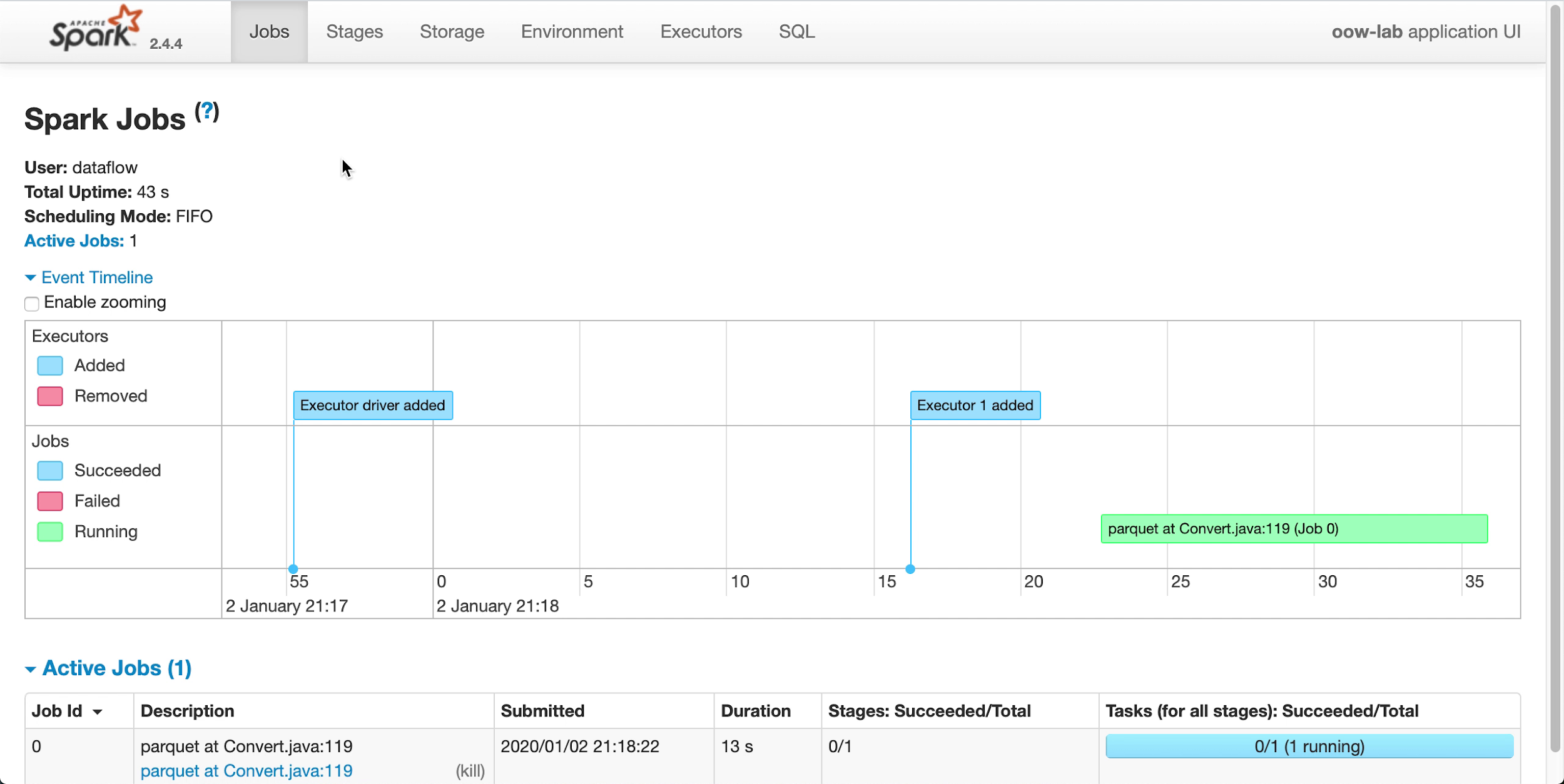
  3. While the Application is running, you can optionally load the Spark UI  to monitor progress. From the Actions menu for the run in question, select Spark UI. The Applications page with Tutorial Example 1 the only application listed. The kebab menu at the end of the row in the list has been clicked, and displays View Details, Edit, Run, Add Tags, View Tags, and Delete. Spark UI is about to be clicked.

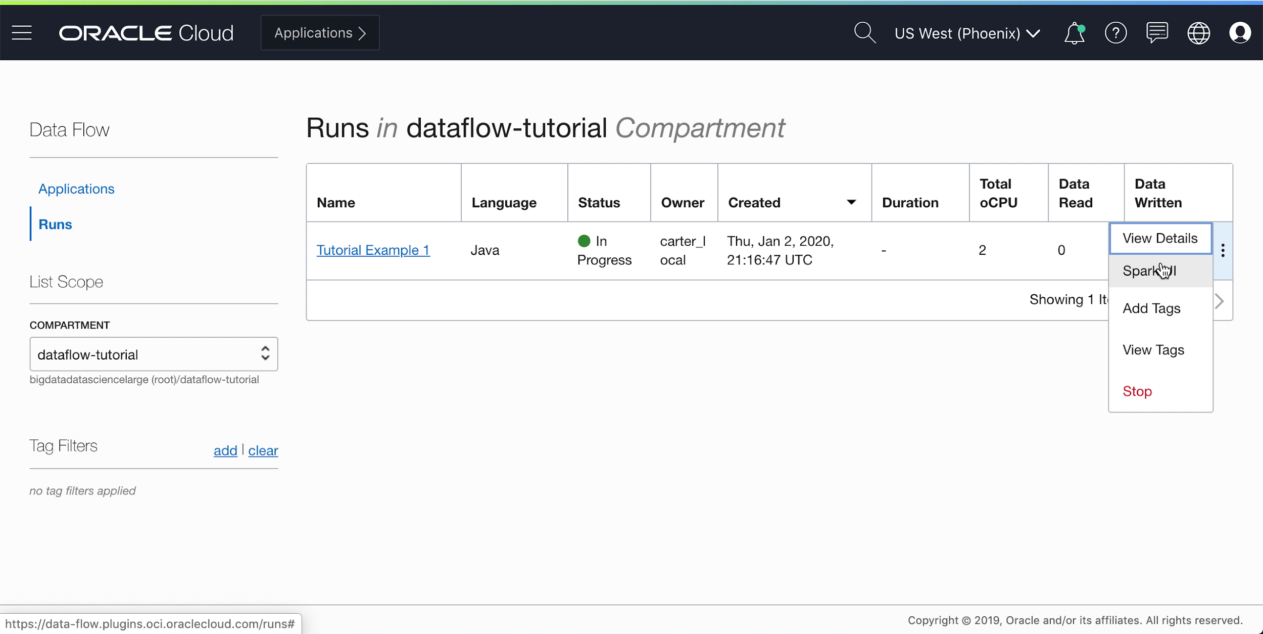
  4. You're automatically redirected to the Apache Spark UI, which is useful for debugging and performance tuning.The Spark UI with a graphic of Executors, when they were added or removed, and Jobs and when they are running and whether they succeeded or failed. They are color-coded. Below is a table of Active jobs, of six columns. The columns are Job ID, Description, Submitted, Duration, Stages: Succeeded/Total, and Tasks (for al stages): Succeeded/Total.
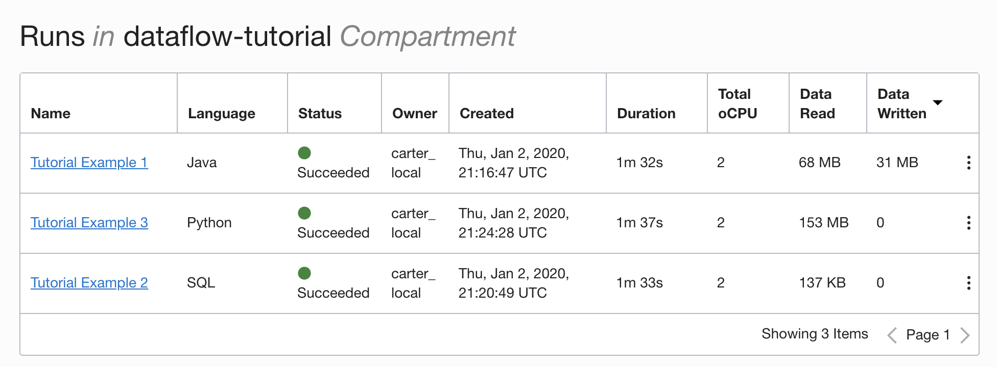
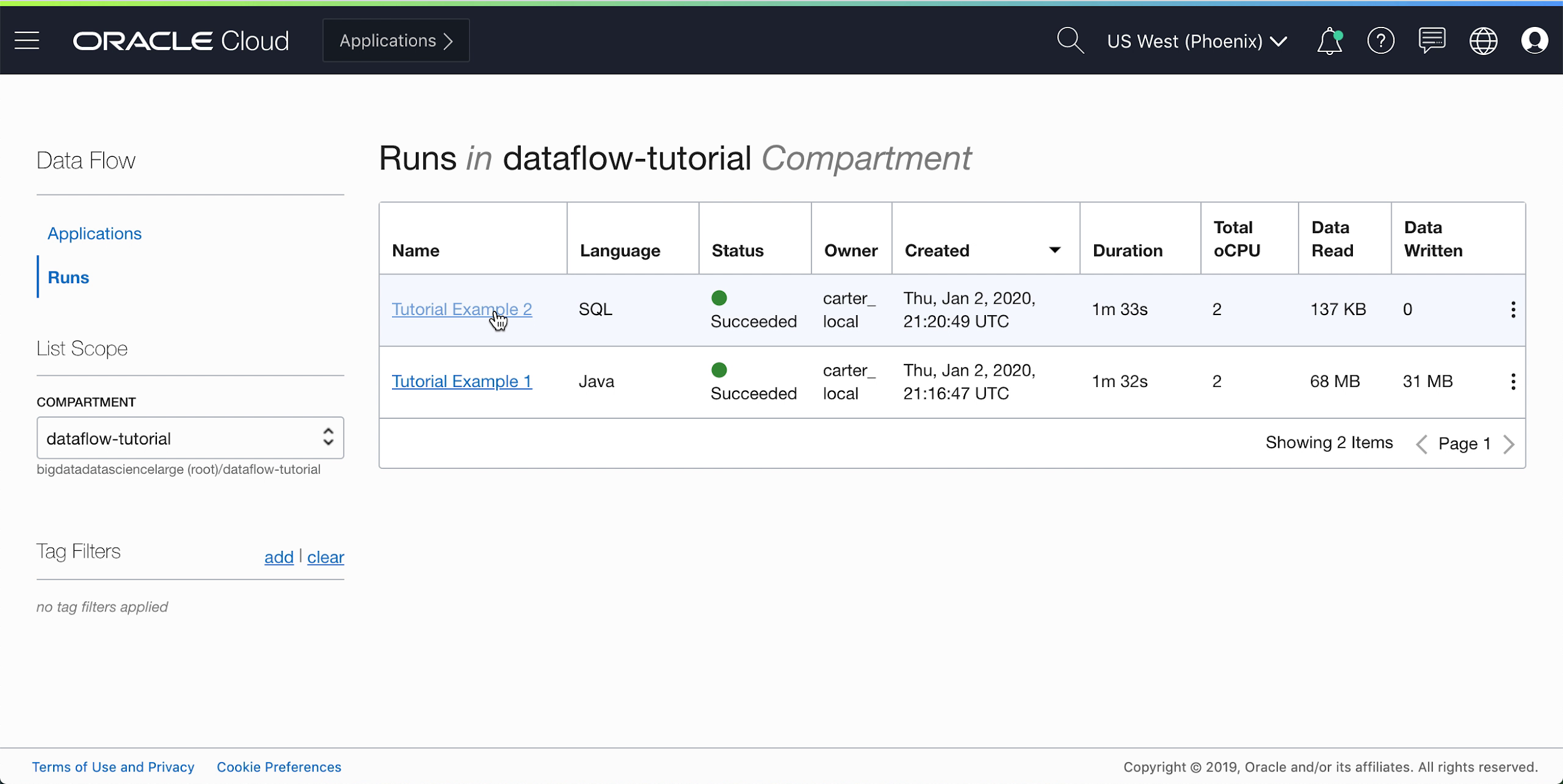
  5. After a minute or so your Run  should show successful completion with a State of Succeeded: The Runs page displayed with two runs, Tutorial Example 1 and Tutorial Example 2, listed. The table of runs has nine columns. They are Name, Language, Status, Owner, Created, Duration, Total oCPU, Data Read, and Data Written. The Status for Tutorial Example 1 is Succeeded.

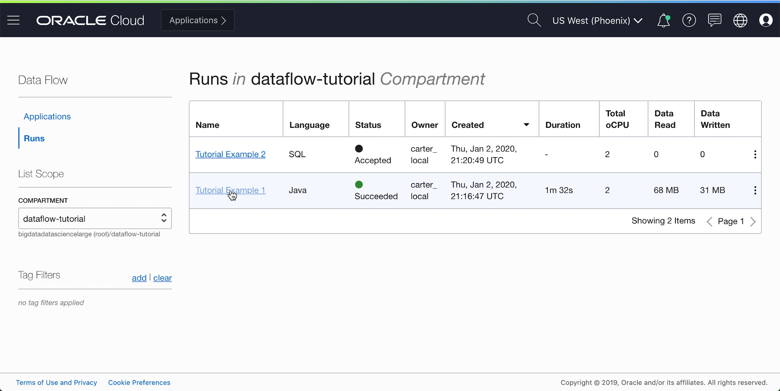
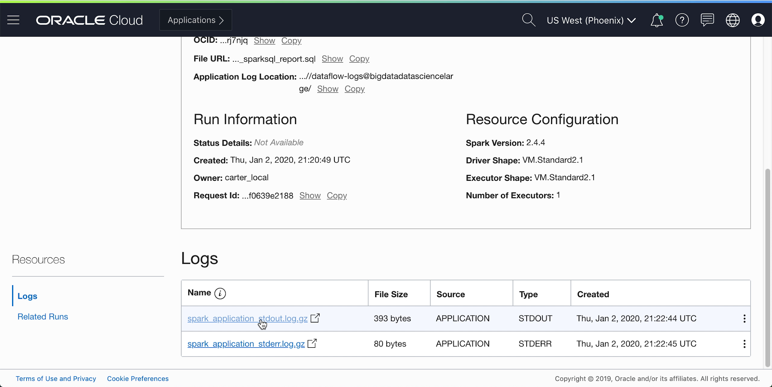
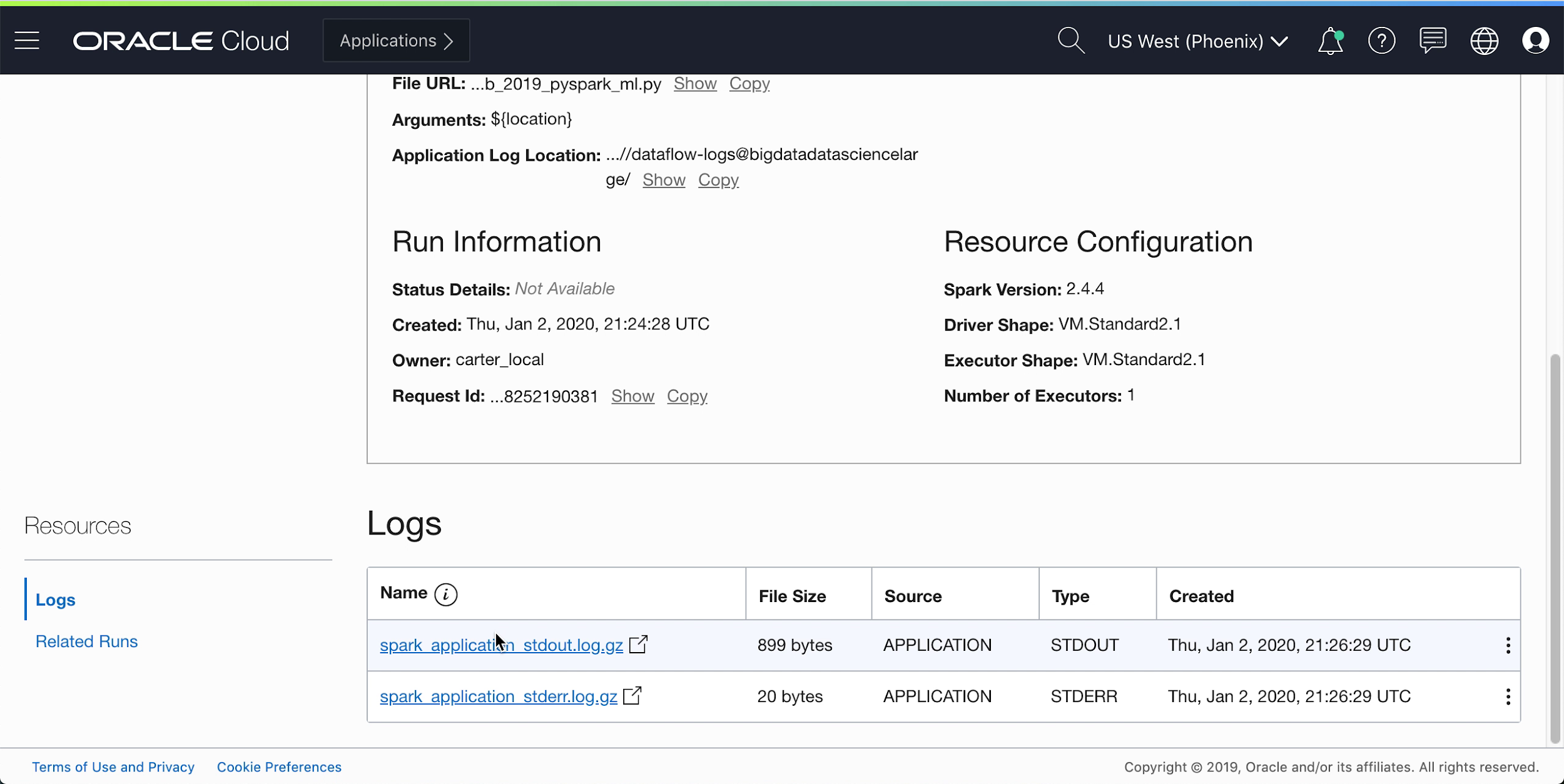
  6. Drill into the Run to see more details, and scroll to the bottom to see a listing of logs. The bottom of the Run Details page containing a section labelled Logs. There is a table of five columns containing two log files. The columns are Name, File Size, Source, Type, and Created. There is a stdout.log file and a stderr.log file. In the left-hand menu to the left of the Logs section is a section called Resources. This contains Logs (which is highlighted as it is selected) and Related Runs.

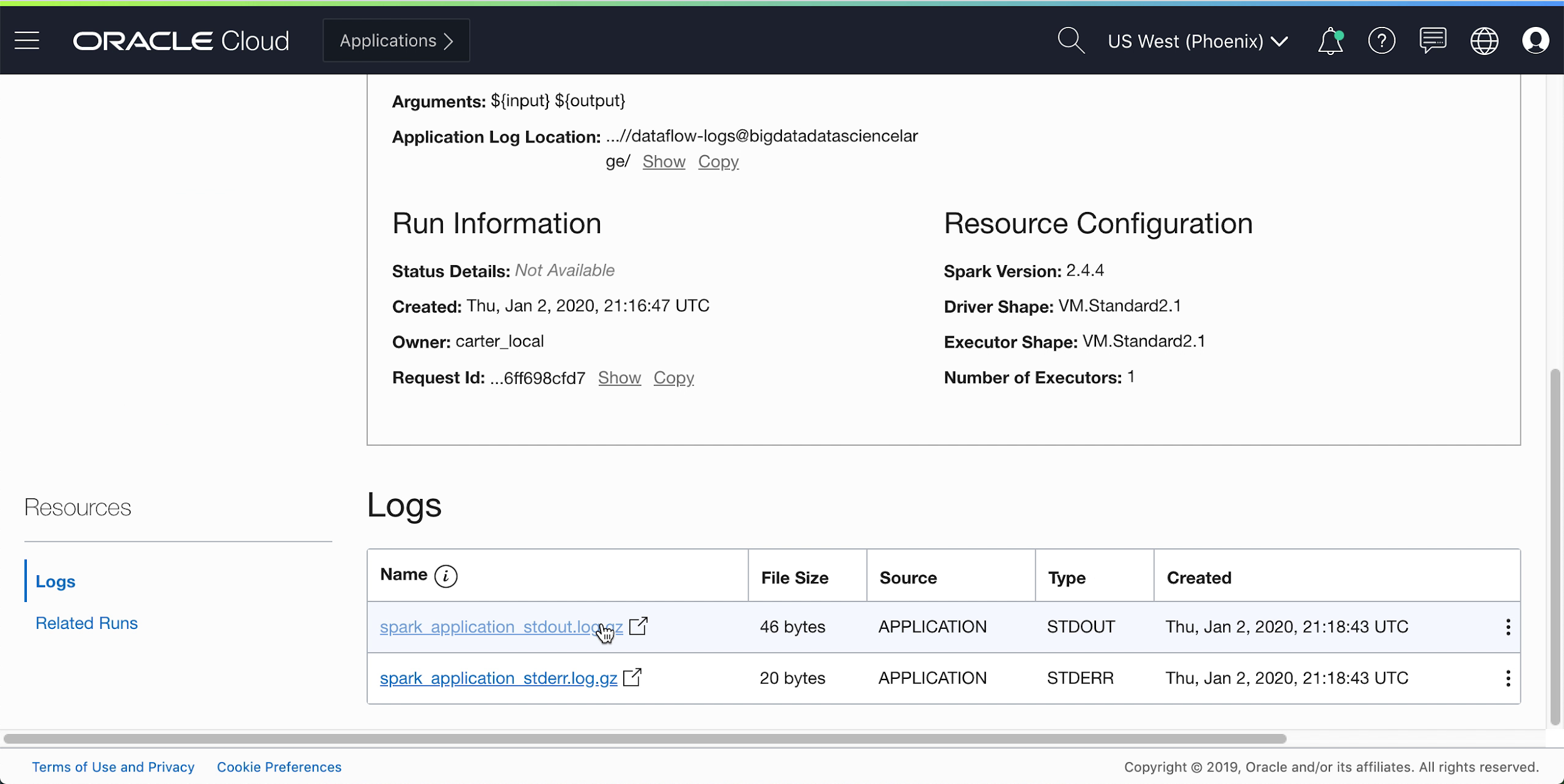
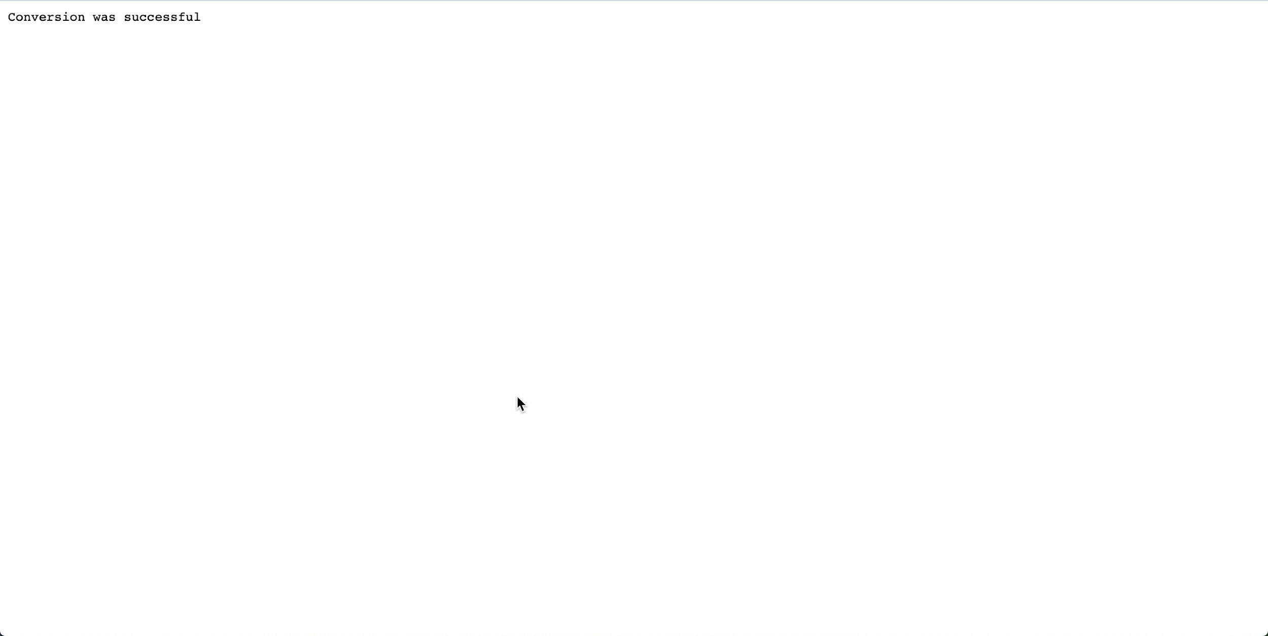
  7. When you click the spark_application_stdout.log.gz file, you should see the following log output: There is a blank page, with some text at the very top. The text is Conversion was successful.

  8. You can also navigate to your output object storage bucket to confirm that new files have been created. The Objects section is displayed. There are three buttons, Upload Objects, Restore, and Delete. Only the first is active. Below is a table of four columns, Name, Size, Status, and Created. the objects available are listed.

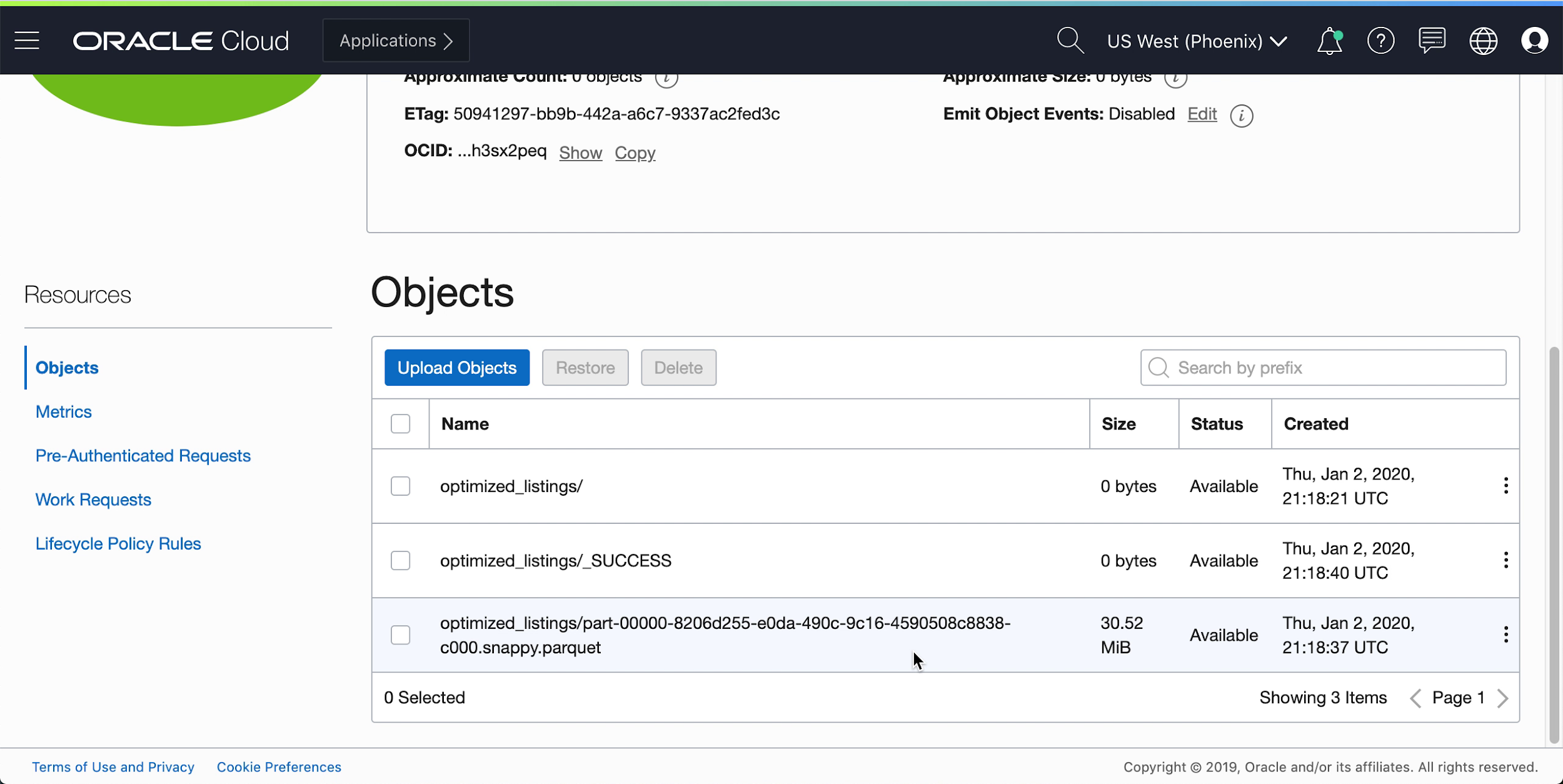
    These new files are used by later applications. Ensure you can see them in your bucket before moving onto the next exercises.

2. SparkSQL Made Simple

In this exercise, you run a SQL script to perform basic profiling of a dataset.

This exercise uses the output you generated in 1. ETL with Java. You must have completed it successfully before you can try this one.

The steps here are for using the Console UI. You can complete this exercise using spark-submit from CLI or spark-submit with Java SDK.

Overview

As with other Data Flow Applications, SQL files are stored in object storage and might be shared among many SQL users. To help this, Data Flow lets you parameterize SQL scripts and customize them at runtime. As with other applications you can supply default values for parameters which often serve as valuable clues to people running these scripts.

The SQL script is available for use directly in the Data Flow Application, you don't need to create a copy of it. The script is reproduced here to illustrate a few points.

Reference text of the SparkSQL Script: Some sample SparkSQL code.

Important highlights:
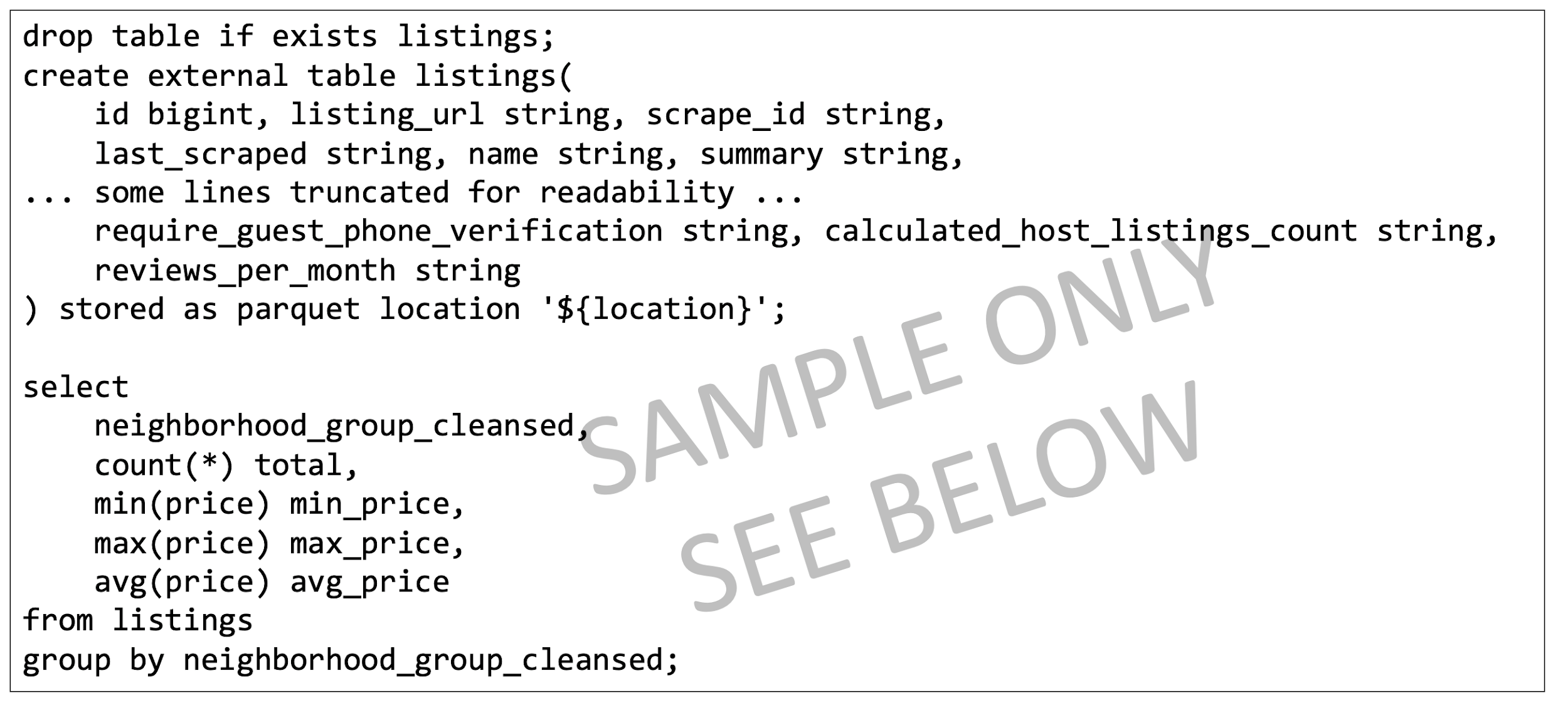
  1. The script begins by creating the SQL tables we need. Currently, Data Flow doesn't have a persistent SQL catalog so all scripts must begin by defining the tables they require.
  2. The table's location is set as ${location} This is a parameter which the user needs to supply at runtime. This gives Data Flow the flexibility to use one script to process many different locations and to share code among different users. For this lab, we must customize ${location} to point to the output location we used in Exercise 1
  3. As we will see, the SQL script's output is captured and made available to us under the Run.
Create a SQL Application
  1. In Data Flow, create a SQL Application, select SQL as type, and accept default resources. In the Create Application pull-out page covering the right-hand side of the Applications page, is a section called Application Configuration. The check boxes, Spark streaming and Use Spark-Submit Options, are not selected. Under a label called Language, are four radio buttons. SQL is selected as the language.
  2. Under Application Configuration, configure the SQL Application as follows:
    1. File URL: is the location of the SQL file in object storage. The location for this application is:
      oci://oow_2019_dataflow_lab@idehhejtnbtc/oow_2019_dataflow_lab/usercontent/oow_lab_2019_sparksql_report.sql
    2. Arguments: The SQL script expects one parameter, the location of output from the prior step. Click Add Parameter and enter a parameter named location with the value you used as the output path in step a, based on the template
      oci://[bucket]@[namespace]/optimized_listings

    When you're done, confirm that the Application configuration looks similar to the following:

    In the Create Application pull-out page covering the right-hand side of the Applications page, the Application Configuration section is visible. There is a check box, Use Spark-Submit Options, not selected. Under Language are four radio buttons, SQL is selected. There is a section called Select a file. In it the check box, Enter the file URL manually, is selected. There is a text box, labelled File URL, which contains the link to the .sql file. Below that are two text boxes side-by-side in the Parameters sub-section. The first is labelled Name, contains location. The second is labelled Value and contains the path to a directory.

  3. Customize the location value to a valid path in your tenancy.
Run a SQL Application
  1. Save the Application and run it from the Applications list. The Applications page with the two applications created so far in this tutorial in reverse chronological order. The table listing the applications contains five columns, Name, Language, Owner, Created, and Updated. At the end of each row is a kebab menu. For Tutorial Example 2, the kebab menu has been clicked and the options are displayed. They are View Details, Edit, Run, Add Tags, View Tags, and Delete. Run is about to be clicked.
  2. After the Run is complete, open the Run: The Runs page with the two applications created so far in this tutorial in reverse chronological order. Each has had on;y one run. The table listing the applications contains nine columns, Name, Language, Status, Owner, Created, Duration, Total oCPU, Data Read, and Data Written. The status of Tutorial Example 2 is Succeeded and the other cells in the table are populated.
  3. Navigate to the Run logs: The bottom of the Run Details page. Below the details is a section labelled Logs. It lists the available log files in a table of five columns. The columns are Name, File Size, Source, Type, and Created. The two log files listed are stdout.log and stderr.log. To the left is a small section labelled Resources. It contains two links, Logs and Resources. Logs is selected.
  4. Open spark_application_stdout.log.gz and confirm that the output agrees with the following output.
    Note

    Your rows might be in a different order from the picture but values should agree.
    The spark_application_stdout.log.gz file output. There are five columns of data. The columns are unnamed and not of consistent width. The first column contains text, the others contain numbers.
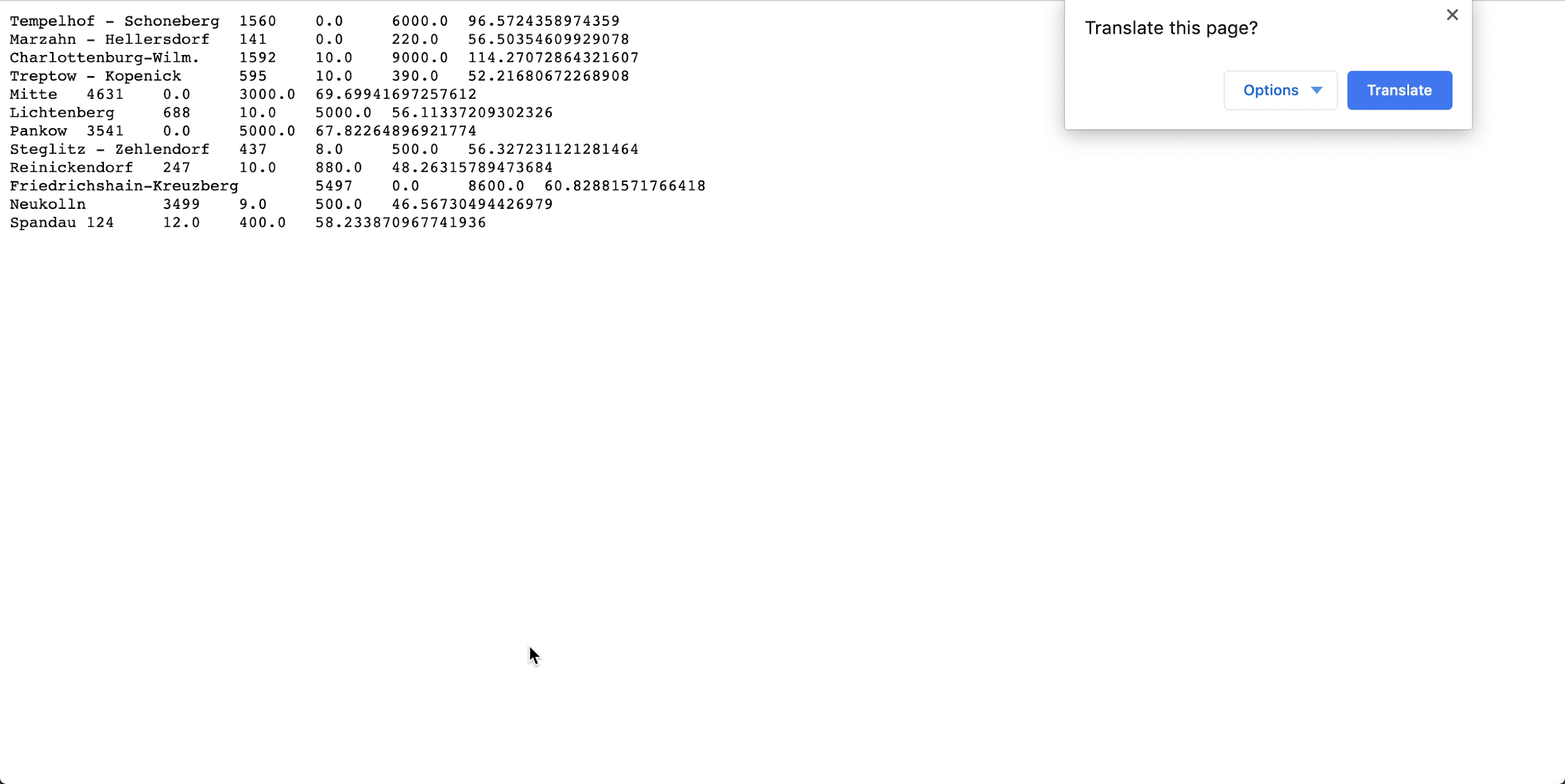
  5. Based on your SQL profiling, you can conclude that, in this dataset, Neukolln has the lowest average listing price at $46.57, while Charlottenburg-Wilmersdorf has the highest average at $114.27 (Note: the source dataset has prices in USD rather than EUR.)

This exercise has shown some key aspects of Data Flow. When a SQL application is in place anyone can easily run it without worrying about cluster capacity, data access and retention, credential management, or other security considerations. For example, a business analyst can easily use Spark-based reporting with Data Flow.

3. Machine Learning with PySpark

Use PySpark to perform a simple machine learning task over input data.

This exercise uses the output from 1. ETL with Java as its input data. You must have successfully completed the first exercise before you can try this one. This time, your objective is to identify the best bargains among the various Airbnb listings using Spark machine learning algorithms.

The steps here are for using the Console UI. You can complete this exercise using spark-submit from CLI or spark-submit with Java SDK.

Overview

A PySpark application is available for you to use directly in your Data Flow Applications. You don't need to create a copy.

Reference text of the PySpark script is provided here to illustrate a few points: Sample PySpark code.

A few observations from this code:
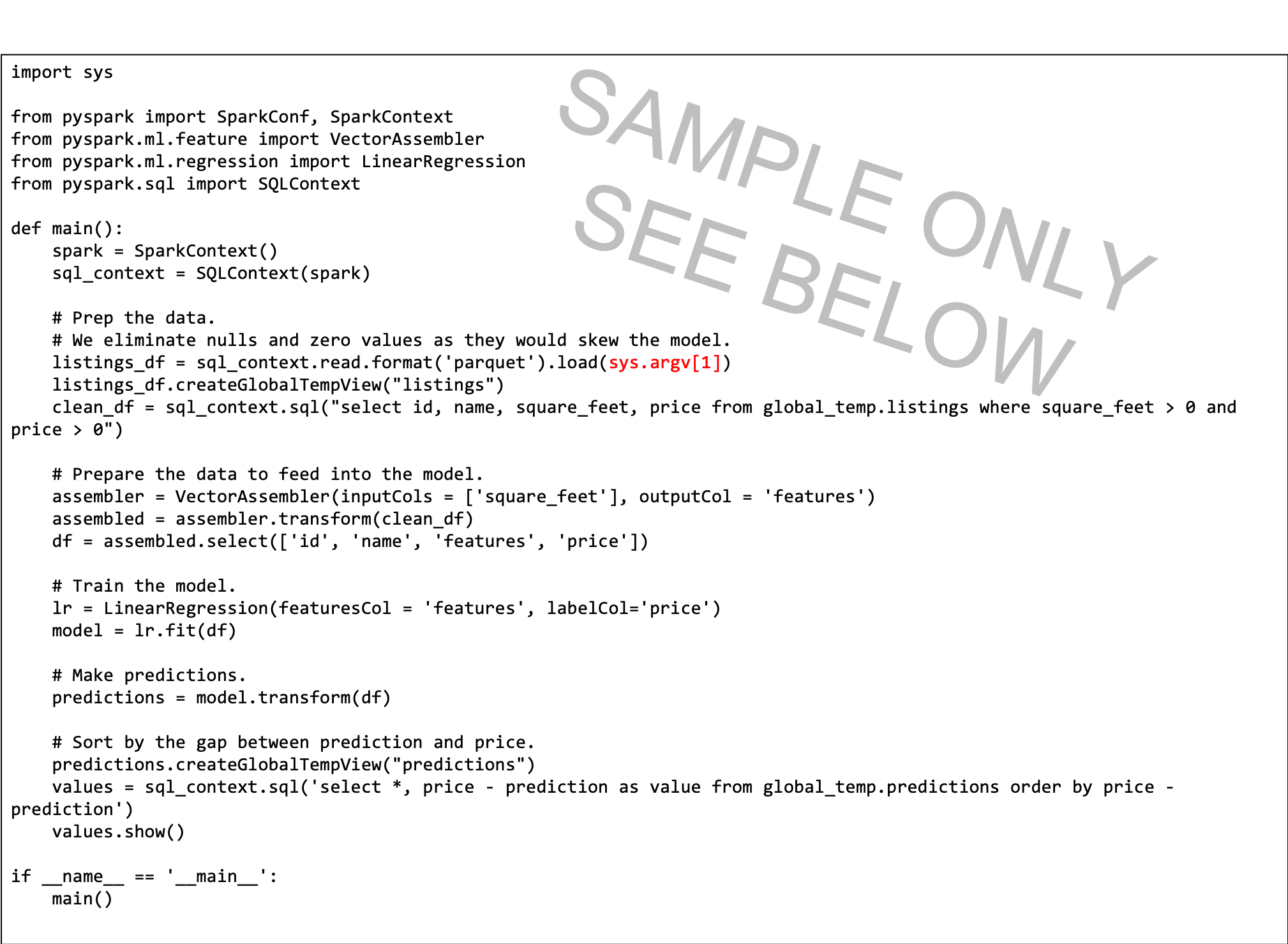
  1. The Python script expects a command line argument (highlighted in red). When you create the Data Flow Application, you need to create a parameter with which the user sets to the input path.
  2. The script uses linear regression to predict a price per listing, and finds the best bargains by subtracting the list price from the prediction. The most negative value indicates the best value, per the model.
  3. The model in this script is simplified, and only considers square footage. In a real setting you would use more variables, such as the neighborhood and other important predictor variables.
Create a PySpark Application

Create a PySpark Application from the Console, or with Spark-submit from the command line or using SDK.

Machine Learning with PySpark Using the Console

Create a PySpark application in Data Flow using the Console.

  1. Create an Application, and select the Python type.
    In the Create Application pull-out page, Python is selected as the language.
  2. In Application Configuration, configure the Application as follows:
    1. File URL: is the location of the Python file in object storage. The location for this application is:
      oci://oow_2019_dataflow_lab@idehhejtnbtc/oow_2019_dataflow_lab/usercontent/oow_lab_2019_pyspark_ml.py
    2. Arguments: The Spark app expects two command line parameters, one for the input and one for the output. In the Arguments field, enter
      ${location}
      . You're prompted for a default value. Enter the value used as the output path in step a on the template:
      oci://<bucket>@<namespace>/optimized_listings
  3. Double-check the Application configuration, and confirm it's similar to the following:
    In the Create Application pull-out page covering the right-hand side of the Applications page, the Application Configuration section is visible. There is a check box called Use Spark-Submit Options, which is not selected. Python is selected as the language. There is a text box, labelled File URL, which contains the link to the .py file. Below is another text box, labelled Arguments, which contains ${location}. Below that are two text boxes side-by-side in the Parameters sub-section. The first is greyed out and contains location. The second contains the path to a directory.
  4. Customize the location value to a valid path in the tenancy.
Machine Learning with PySpark Using Spark-Submit and CLI

Create a PySpark application in Data Flow using Spark-submit and CLI.

  1. Complete exercise Create the Java Application Using Spark-Submit and CLI, before trying this exercise. The results are used in this exercise.
  2. Run the following code:
    oci --profile <profile-name> --auth security_token data-flow run submit \
    --compartment-id <compartment-id> \
    --display-name Tutorial_3_PySpark_ML \
    --execute '
        oci://oow_2019_dataflow_lab@idehhejtnbtc/oow_2019_dataflow_lab/usercontent/oow_lab_2019_pyspark_ml.py 
        oci://<your_bucket>@<namespace-name>/output/tutorial1'
Machine Learning with PySpark Using Spark-Submit and SDK

Create a PySpark application in Data Flow using Spark-submit and SDK.

  1. Complete exercise Create the Java Application Using Spark-Submit and SDK, before trying this exercise. The results are used in this exercise.
  2. Run the following code:
    public class PySParkMLExample {
     
      private static Logger logger = LoggerFactory.getLogger(PySParkMLExample.class);
      String compartmentId = "<compartment-id>"; // need to change comapartment id
     
      public static void main(String[] ars){
        System.out.println("ML_PySpark Tutorial");
        new PySParkMLExample().createRun();
      }
     
      public void createRun(){
     
        ConfigFileReader.ConfigFile configFile = null;
        // Authentication Using config from ~/.oci/config file
        try {
          configFile = ConfigFileReader.parseDefault();
        }catch (IOException ie){
          logger.error("Need to fix the config for Authentication ", ie);
          return;
        }
     
        try {
        AuthenticationDetailsProvider provider =
            new ConfigFileAuthenticationDetailsProvider(configFile);
     
        DataFlowClient client = new DataFlowClient(provider);
        client.setRegion(Region.US_PHOENIX_1);
     
        String executeString = "oci://oow_2019_dataflow_lab@idehhejtnbtc/oow_2019_dataflow_lab/usercontent/oow_lab_2019_pyspark_ml.py oci://<bucket-name>@<namespace-name>/output/optimized_listings";
     
        CreateRunResponse response;
     
        CreateRunDetails runDetails = CreateRunDetails.builder()
            .compartmentId(compartmentId).displayName("Tutorial_3_ML_PySpark").execute(executeString)
            .build();
     
        CreateRunRequest runRequest = CreateRunRequest.builder().createRunDetails(runDetails).build();
        CreateRunResponse response = client.createRun(runRequest);
     
        logger.info("Successful run creation for ML_PySpark with OpcRequestID: "+response.getOpcRequestId()
            +" and Run ID: "+response.getRun().getId());
     
        }catch (Exception e){
          logger.error("Exception creating run for ML_PySpark ", e);
        }
     
     
      }
    }
Run a PySpark Application
  1. Run the Application from the Application list. The Applications page with the three applications created in this tutorial in reverse chronological order. The table listing the applications contains five columns, Name, Language, Owner, Created, and Updated. At the end of each row is a kebab menu. For Tutorial Example 3, the kebab menu has been clicked and the options are displayed. They are View Details, Edit, Run, Add Tags, View Tags, and Delete. Run is about to be clicked.
  2. When the Run completes, open it and navigate to the logs. The bottom of the Run Details page. Below the details is a section labelled Logs. It lists the available log files in a table of five columns. The columns are Name, File Size, Source, Type, and Created. The two log files listed are stdout.log and stderr.log. To the left is a small section labelled Resources. It contains two links, Logs and Resources. Logs is selected.

  3. Open the spark_application_stdout.log.gz file. Your output should be identical to the following: The spark_application_stdout.log.gz file output. There is a table of six columns. The columns are id, name, features, price, prediction, and value. Only the first twenty rows are displayed. All the cells are populated.
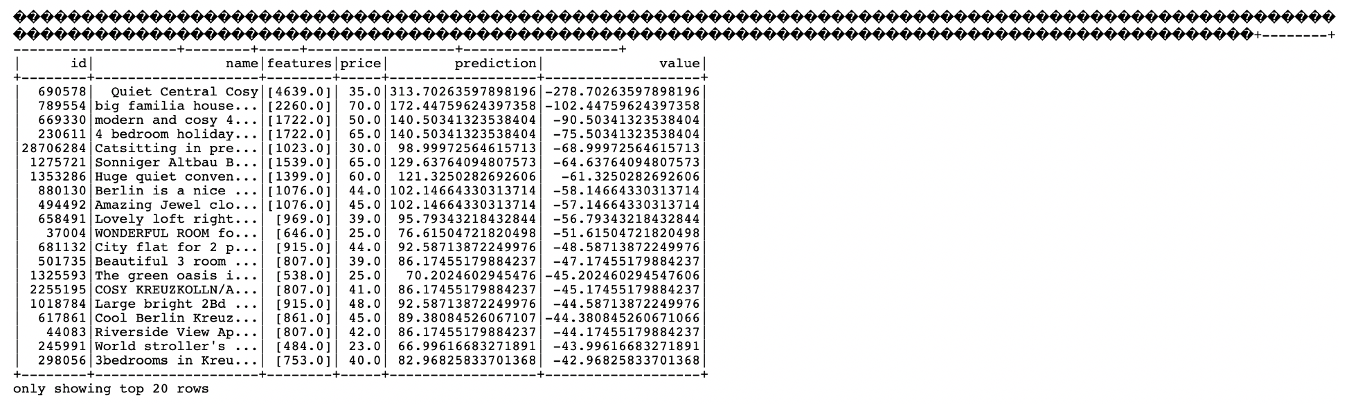
  4. From this output, you see that listing ID 690578 is the best bargain with a predicted price of $313.70, compared to the list price of $35.00 with listed square footage of 4639 square feet. If it sounds a little too good to be true, the unique ID means you can drill into the data, to better understand if it really is the steal of the century. Again, a business analyst could easily consume the output of this machine learning algorithm to further their analysis.

What's Next

Now you can create and run Java, Python, or SQL applications with Data Flow, and explore the results.

Data Flow handles all details of deployment, tear down, log management, security, and UI access. With Data Flow, you focus on developing Spark applications without worrying about the infrastructure.